Sonar Avoidance: An Alternative to Traditional RVO
Sonar Avoidance
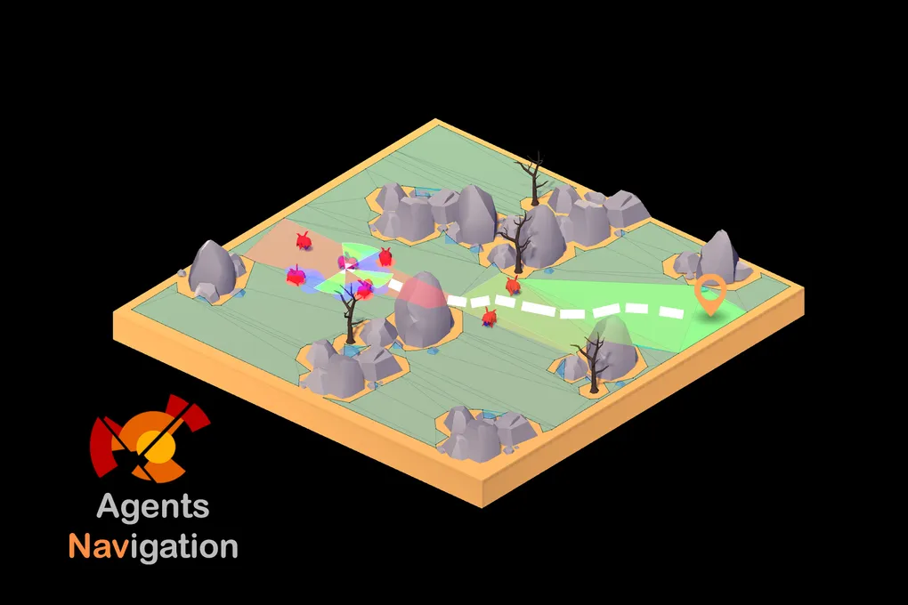
Sonar Avoidance is a local avoidance algorithm for RTS agents that I created for my own game. It is typically combined with a global navigation solution (e.g., a navigation mesh), which provides waypoints, while the algorithm locally avoids obstacles in order to reach those waypoints. It is inspired by StarCraft II and the GDC 2011 talk AI Navigation: It’s Not a Solved Problem - Yet.
In this article, I will cover the history of how I developed the algorithm and explain in detail how it works.
For those interested, Sonar Avoidance is available on the Unity Asset Store as a standalone local avoidance solution under Local Avoidance as well as with full Unity NavMesh integration under Agents Navigation. Since 2022, these packages have been downloaded approximately 23,000 times and have been successfully used in several released games, indicating strong demand for a more game-ready navigation solution.
History of the Algorithm
In this section I will cover the motivation behind the algorithm and how it evolved. If you are mainly interested in technical details, you can skip this section.
Warcraft
In 2014, I started working with Unity. It was there that I discovered the engine as a powerful tool for creating games. I quickly fell in love with the tool and decided that I want to create the game with it. This then I started developing my wacraft 3 mobile knock-off.
Looking back, directly copying Warcraft III, even for mobile, was not the best idea. Without Blizzard’s approval, it would never have been possible to release it officially. At the time, though, I genuinely hoped Blizzard might see the project and become interested. That never happened, but I did try.
A significant part of my teenage years was spent modding Warcraft III maps, experimenting with mechanics and building custom experiences. Creating this project in Unity felt like a continuation of that journey, inspired by the World Editor, which was incredibly powerful and, in my opinion, one of Blizzard’s greatest creations.
Navigation Solution
One of the most important features of any RTS game is agent navigation. If it does not feel right, players quickly become frustrated.
In RTS games, movement is a core gameplay mechanic, not just a way to travel between points. Units are constantly redirected, split, grouped, and micro-managed under pressure. If they get stuck, jitter, block each other, or take visibly poor paths, the game feels unreliable and unresponsive.
Good navigation becomes invisible. Units flow naturally around obstacles, surround targets efficiently, and execute commands precisely. For this reason, navigation is not just a technical system but a fundamental part of game feel and competitive integrity.
Unity Navigation
Since I was building the game in Unity, I initially used their built-in solution. It consisted of global navigation using a navigation mesh and local avoidance using ORCA.
A Navigation Mesh or navmesh is a triangulated representation of walkable areas in the game world. Obstacles are excluded from the mesh. Pathfinding is typically performed using the A* Search Algorithm between start and destination nodes.
NavMesh generation is expensive, but it produces far fewer nodes than grid-based systems. Because rebuilding is costly, it is generally used only for static obstacles such as buildings.
For dynamic avoidance between moving agents, Unity used ORCA. ORCA is an extension of RVO designed to provide more accurate multi-agent avoidance.
In many scenarios, ORCA works very well. It produces convincing crowd behavior and handles dense group motion nicely. However, in RTS-style gameplay, several limitations became apparent in practice when using Unity’s default configuration.
Problems with ORCA
The first major issue appeared in classic RTS situations where units try to surround a target.
In Unity’s default implementation at the time, agents often clumped on one side instead of properly distributing themselves around the target. In games like Warcraft III, where each unit is important, this is unacceptable because some units would simply stand idle instead of attacking.
The second issue was ORCA’s reliance on velocity modulation. This makes sense in crowd simulations, and there are many papers explaining how density-based velocity adjustment performs well in high congestion scenarios.
However, in RTS games, high congestion is less frequent and large groups often move toward objectives. In such cases, reducing velocity becomes a drawback because units no longer maximize their speed. If you are micro-managing a single unit, you do not want it to slow down unnecessarily just to accommodate nearby agents.
The third issue was ORCA’s difficulty escaping concave formations. Agents entering these situations could become permanently stuck.
After encountering these problems, I concluded that NavMesh combined with the default ORCA setup would not be sufficient for the gameplay feel I wanted.
Researching Alternatives
Around 2016 it was surprisingly difficult to find detailed information about navigation systems used in successful RTS games. Most information was sparse and surface level.
My assumption was that navigation quality plays a major role in RTS success, so companies treated their solutions as proprietary. That may or may not be true, but public technical information was limited.
Warcraft III Navigation
The obvious first reference was Warcraft III.
From my investigation, Warcraft III used a grid-based solution for both global navigation and local avoidance.
In grid-based navigation, the world is divided into fixed-size nodes. Each node indicates whether it is traversable. Agents run A* Search Algorithm to find a sequence of nodes connecting start and destination.
In Warcraft III, army sizes were usually limited by resource caps. However, when those limits were removed using the editor, performance degraded significantly. Groups of 100 or more units began blocking each other, jittering, and behaving poorly.
The main limitation was the discrete nature of the system. It lacked the fluid motion seen in StarCraft II.
Although I was recreating Warcraft III style gameplay, I wanted better navigation quality, so I decided against using a purely grid-based approach.
Supreme Commander 2 Navigation
Another game that impressed me even more in terms of large-scale movement was Supreme Commander 2.
Large armies could pass through each other with very fluid motion.
From research I found they were using a modified version of Continuum Crowds. It is a grid-based approach that uses flow fields.
In a flow field, each grid node stores a direction guiding agents toward a shared goal. Instead of each agent computing an individual path, the environment provides a velocity field.
You can imagine the field as an ocean and the goal as a vortex. No matter where you place the agent, it flows toward the destination.
Continuum Crowds incorporates density and velocity information to produce highly fluid group motion.
The main limitation of flow fields is that path calculation happens for shared goals across the whole graph. This makes them extremely efficient for large groups with the same objective, but inefficient when many agents have different goals or when maps are very large.
Supreme Commander 2 was clearly designed around this limitation. Large groups share goals and there are fewer individually controlled units. In Warcraft-style games you have many independent agents such as workers, heroes, and neutral units.
StarCraft II Navigation
Eventually I returned to StarCraft II. To this day, StarCraft II is widely considered one of the best navigation implementations in RTS games. It was done so well that some professional players disliked it because it reduced the mechanical difficulty of unit control that was very relevant in StarCraft I.
Finding reliable information about its navigation system was challenging. Blizzard kept technical details minimal.
Through experimentation and observation, I concluded that StarCraft II used NavMesh for global navigation and a proprietary local avoidance solution.
The only meaningful public source I found was the GDC 2011 talk AI Navigation: It’s Not a Solved Problem - Yet.
The talk focused more on design challenges than technical implementation. They confirmed NavMesh usage and explained how they handled rebuilding efficiently. Their solution appeared simpler and more 2.5D-focused compared to Unity’s more general 3D NavMesh.
The key hint about avoidance was that it behaved almost like a vision-based system. Agents seemed to look ahead, detect openings, and steer through available gaps.
That observation became the foundation of what later evolved into Sonar Avoidance.
Algorithm
Analogy to Human Vision
The Sonar Avoidance Algorithm can be understood through a simple human analogy. When people walk forward, they perceive the world as a forward-facing field of view centered around where they are looking. Static obstacles visually occupy a portion of that field. If something appears slightly to the left or right, we instinctively avoid walking into the angular region it occupies. In other words, obstacles “block” parts of our visual space, and we naturally choose a direction outside those blocked angles.
For moving obstacles, humans go one step further. We do not react only to where someone is, but also to where they are going. Subconsciously, we predict whether our current walking direction would intersect with their future path. If it would, we slightly adjust our heading so the projected trajectories no longer collide.
The algorithm mirrors this behavior mathematically. It treats perception as an angular field centered at
Overview
The Sonar Avoidance Algorithm is a 1D angular-space local avoidance method.
Instead of solving constraints directly in velocity space, the algorithm projects obstacles into angular intervals and subtracts blocked regions from the agent’s field of view.
The result is a set of safe steering angles from which the optimal direction is selected.
High-Level Pseudocode
function ComputeSteering(agent):

    desiredDir = GetDesiredDirectionFromNavMesh(agent)
    Θ = [ [-θ_max, 0], [0, θ_max] ]   // two initial vision intervals

    obstacles = CollectObstaclesWithinHorizon(agent)

    blockedIntervals = []

    for each staticObstacle:
        interval = BuildStaticInterval(agent, staticObstacle, desiredDir)
        blockedIntervals.add(interval)

    for each dynamicObstacle:
        interval = BuildDynamicInterval(agent, dynamicObstacle, desiredDir)
        blockedIntervals.add(interval)

    for each wallSegment:
        interval = BuildWallInterval(agent, wallSegment, desiredDir)
        blockedIntervals.add(interval)

    safeIntervals = SubtractIntervals(Θ, blockedIntervals)

    θ* = ArgMinCost(safeIntervals, desiredAngle=0, velocityAngle)

    return DirectionFromAngle(θ*)
Agent Model
Each agent is defined as:
- Position:
- Velocity:
- Radius:
- Horizon:
radius of sonar volume - Preferred speed:
From global navigation, the agent receives a desired direction:
Angular Space Representation
The angular domain is represented as two separate intervals:
Where:
corresponds to desired direction. - Negative angles represent left.
- Positive angles represent right.
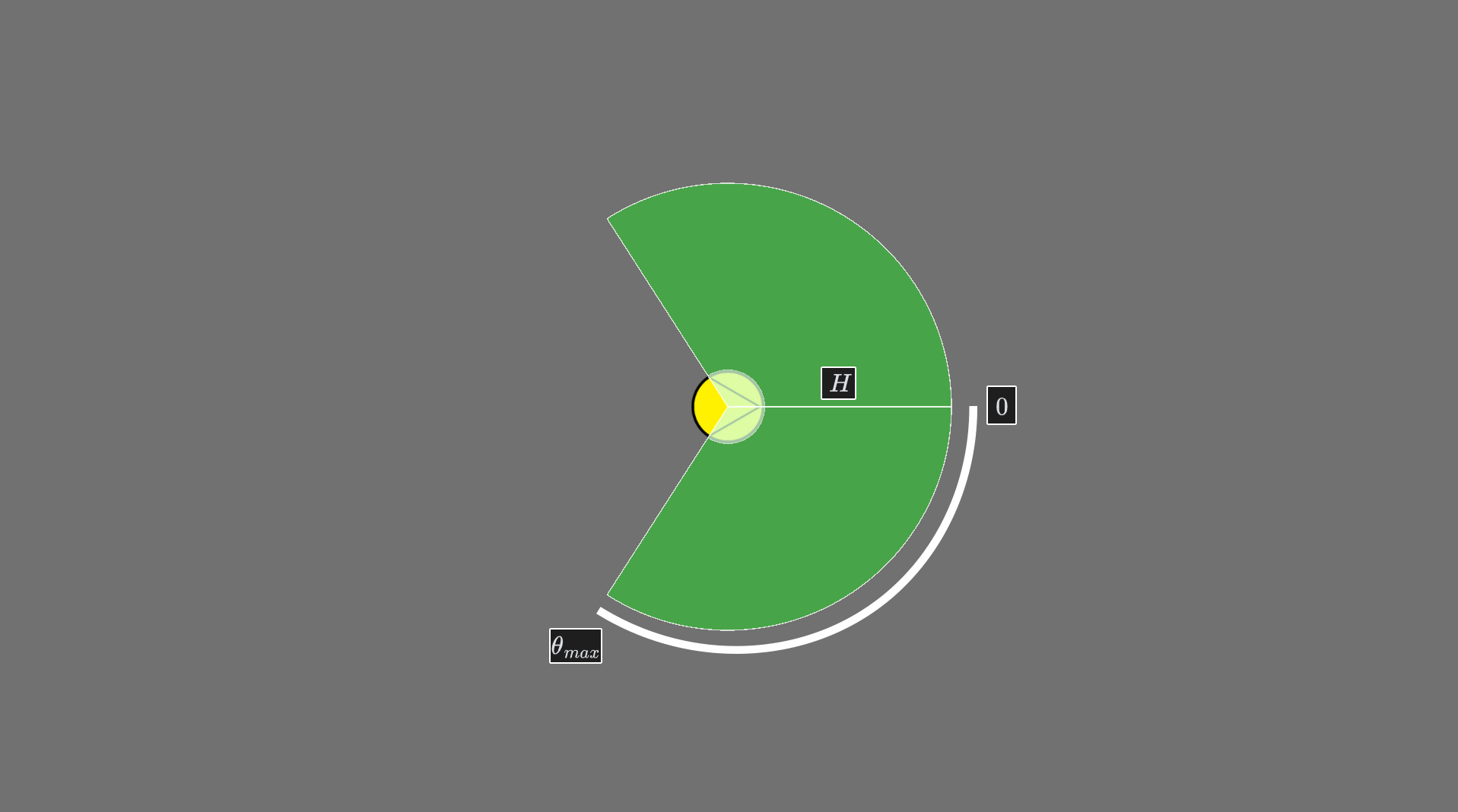 Figure 1: The yellow circle represents the agent, and the two green sections represent the sonar detection volume.
Local Space Transformation
All computations are performed in the agent’s local coordinate frame, defined such that:
- The agent is at the origin.
- The desired direction aligns with the positive x-axis.
Let the agent position be:
and the normalized desired direction:
We define a rotation function:
such that
For any world-space point
For any world-space velocity or direction vector
After transformation, the desired direction becomes:
Since RTS movement is typically planar (e.g., XZ), all angular computations operate on the 2D components of
Static Obstacles
Static obstacle:
- Position:
- Radius:
After transforming to local space:
Let:
Distance to obstacle center:
If
Otherwise, we compute its angular span
Central angle:
Angular half-width:
Blocked interval:
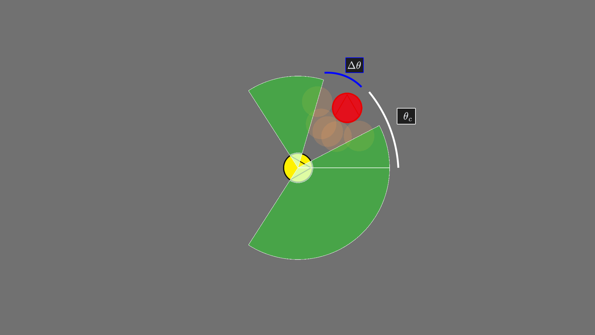 Figure 2: The red circle represents the obstacle, and the orange circles indicate where the agent would collide if it moved in directions toward the obstacle.
Dynamic Obstacles
Each dynamic obstacle is defined as:
- Position:
- Velocity:
- Radius:
After transforming to agent-local space:
As we are trying to find all
Collision condition:
Whereas we only care about dynamic obstacles that are within the sonar volume:
Solving the equation for
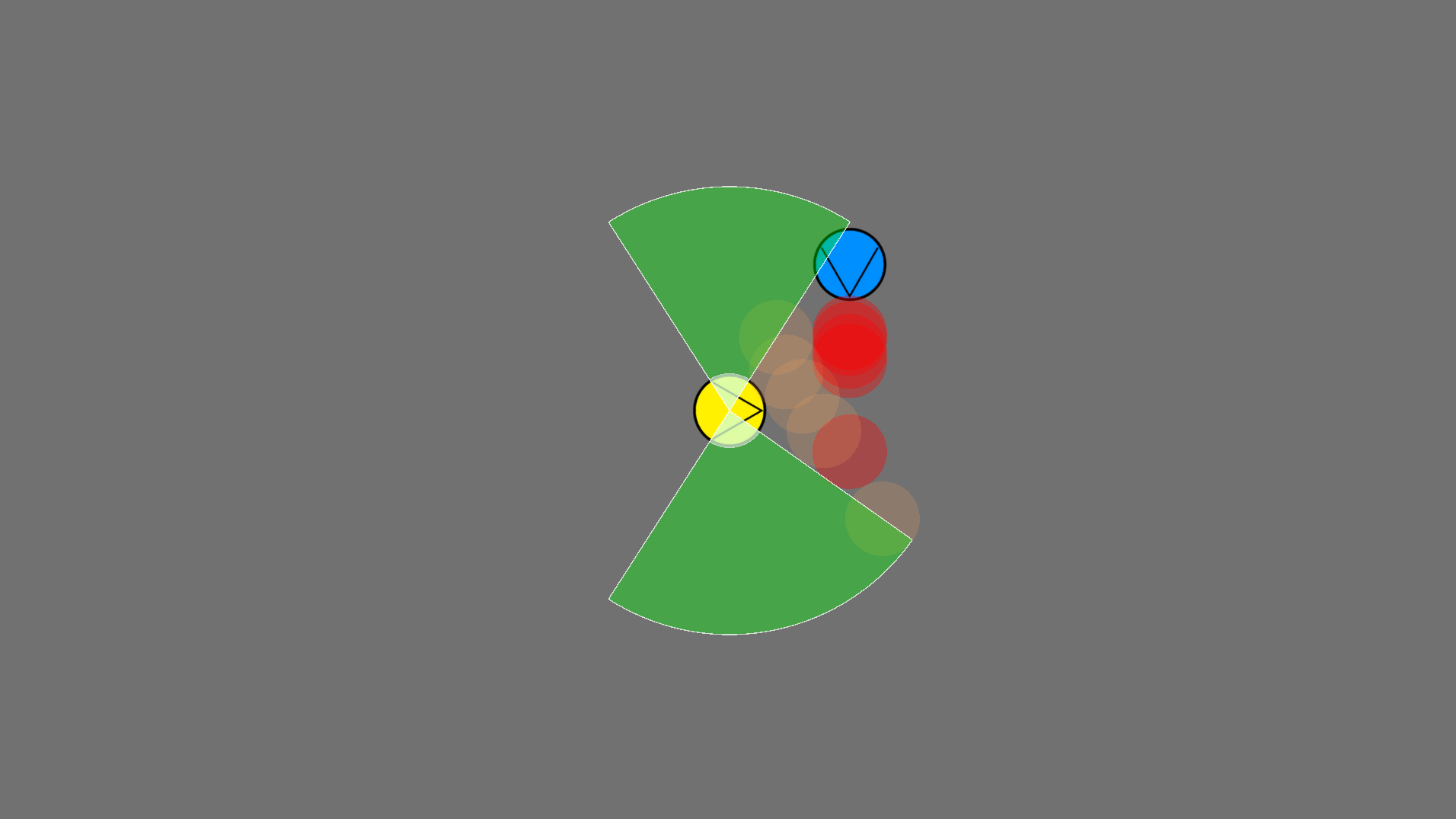 Figure 3: The obstacle is moving downward at a speed of 2, and the agent is moving to the right at a speed of 1. The red circles show how the algorithm predicts all possible collision angles. It chooses to move toward the obstacle’s current position because, by the time the agent reaches it, the obstacle will have already moved away.
NavMesh Walls
Each wall segment is defined as:
- Start:
- End:
- Radius is not required, as a typical NavMesh is already built to account for the agent’s radius
After transformation:
The wall is treated as a line segment obstacle. We compute angular span of both endpoints:
The span between them becomes a blocked interval:
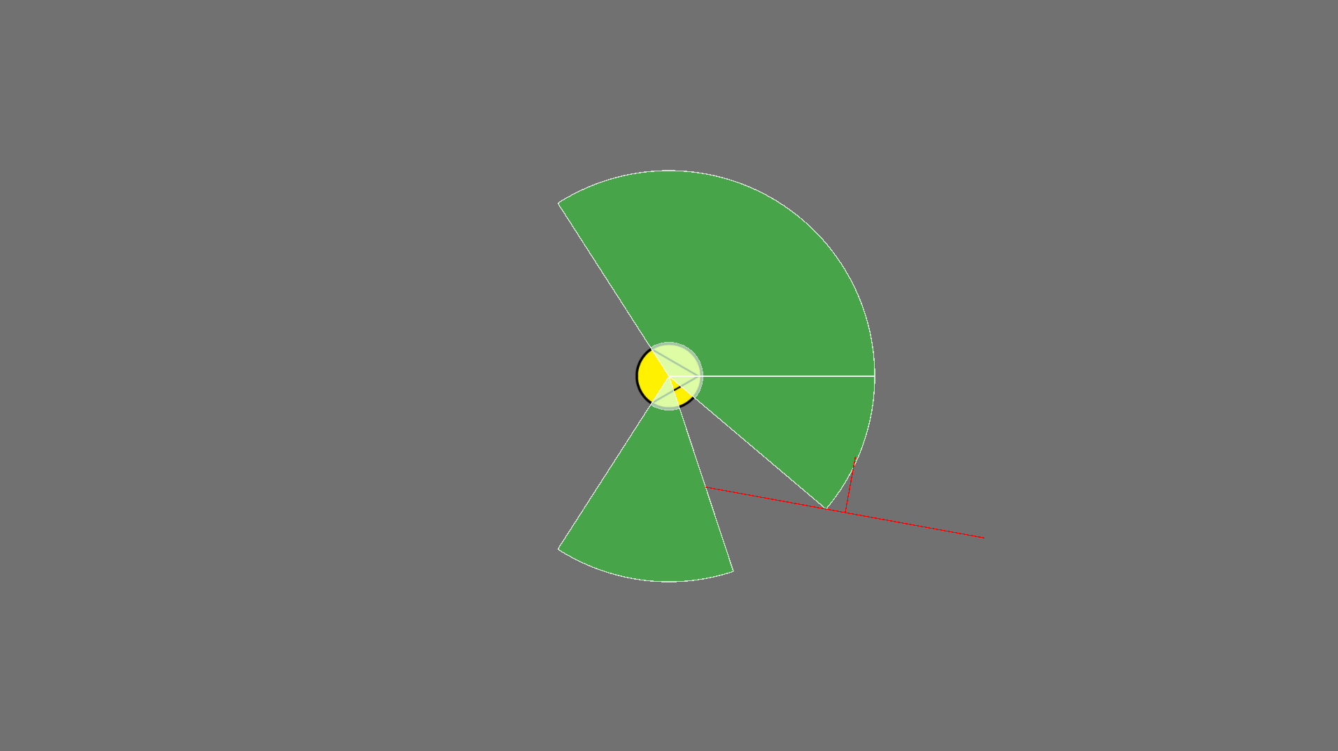 Figure 4: The yellow circle represents the agent, and red line the navmesh wall.
Interval Subtraction
All blocked intervals are collected:
Safe space is computed by subtracting blocked intervals from vision space:
Result:
If no safe interval remains, a fallback strategy is required (for example, selecting the minimal-penetration angle or temporarily reducing speed) to avoid deadlock.
Direction Selection
From safe intervals
We define:
- Desired angle:
- Current velocity angle:
Cost function:
Where:
controls preference toward goal direction. controls smoothness / inertia.
Optimization:
Steering Output
Final steering direction in local space:
Transformed back to world space:
This direction is used for velocity steering.
Smart Stop
The algorithm typically terminates when the agent is sufficiently close to its destination.
However, like most local avoidance algorithms, Sonar Avoidance does not guarantee convergence in all configurations.
In particular, purely local steering can result in oscillations or non-convergent behavior when agents compete for the same spatial region.
Therefore, a higher-level termination mechanism is required to detect pathological cases and terminate movement safely.
Two simple strategies are sufficient to handle most remaining scenarios.
We call them Hive Mind Stop and Give Up Stop.
Hive Mind Stop
Hive Mind Stop addresses termination during coordinated group movement.
When multiple agents move toward the same destination (for example, surrounding a target), typically one agent reaches the final position first.
The remaining agents may continue oscillating around the destination without finding an exact collision-free configuration.
To stabilize termination, each agent that is within a small threshold distance from the destination performs an additional check:
- Inspect nearby dynamic obstacles.
- If neighboring agents are:
- Already stopped,
- Have a similar destination,
- And are within a small proximity threshold,
then the agent also terminates movement.
Effectively, termination propagates through the group once sufficient spatial coverage is achieved.
This produces stable and visually coherent group stopping behavior while avoiding persistent micro-oscillation near the goal.
Figure 5: Left: agents attempt to reach a single-point destination. Once one agent occupies the space, the others circle indefinitely. Right: with Hive Mind Stop enabled, agents immediately terminate once the first agent stops, as the stop state propagates through the group.
Give Up Stop
Give Up Stop handles situations where an agent becomes stuck in complex concave obstacle formations or prolonged deadlock.
Each agent maintains a bounded timer:
Initialization:
At each simulation step with timestep
If blocking conditions persist, the timer increases:
If forward progress resumes, the timer decreases:
If
the agent terminates movement.
Figure 6: During formation movement, an agent’s assigned destination can become obstructed and effectively unreachable. While some games (e.g., StarCraft II) use push-out mechanics to alleviate congestion, this does not prevent deadlock when agents are holding position. Left: the agent circles indefinitely because its destination is unreachable. Right: the Give Up Stop mechanism terminates movement after a bounded time.
Complexity Analysis
Let:
= total number of agents in the system = static obstacles within sonar horizon = dynamic obstacles within sonar horizon = wall segments intersecting the sonar volume
Let:
For a single agent, interval construction requires:
Since the angular domain is 1D and bounded, interval clipping and subtraction are linear in the number of nearby obstacles.
System-wide complexity therefore becomes:
where
Local Neighborhood Assumption
In practice, agents only consider obstacles inside the sonar horizon
This ensures that
Using spatial partitioning structures (e.g., grids or trees), neighborhood queries can be treated as approximately constant time on average, keeping
Nearest-Obstacle Limiting
In many practical RTS scenarios, it is sufficient to limit the number of processed obstacles:
- Static obstacles: consider only the
nearest. - Dynamic obstacles: consider only the
nearest. - Wall segments: typically all intersecting segments within the sonar horizon must be considered to preserve correctness.
With such limits:
If
Thus, overall system complexity approaches:
In practice, limiting
Result
ORCA / RVO
- Operate in full 2D velocity space.
- Construct half-plane constraints.
- Solve linear program per agent.
- Guarantee reciprocal collision avoidance.
- Complexity depends on constraint solving.
Sonar Avoidance
- Reduces problem to 1D angular space.
- Uses interval subtraction instead of half-plane intersection.
- Avoids linear programming.
- Naturally integrates static geometry and navmesh walls.
- Easier SIMD/ECS optimization.
- Lower constant factors.
Trade-offs:
- Does not guarantee strict reciprocity like ORCA.
- Works best when desired direction dominates behavior.
- More heuristic but computationally simpler.
Figure 7: Circling scenario. Yellow agents use Sonar Avoidance to surround the red obstacle and quickly distribute themselves by searching for available openings. The last agent continues circling because no space remains. Blue agents use Unity ORCA and immediately clump on one side of the obstacle instead of attempting a full surround. In both variations, the destination is offset by the combined radii of the agent and the target, and agents stop upon reaching it.
Figure 8: Concave blockage scenario. The yellow agent uses Sonar Avoidance and attempts to escape the concave trap. Once its visibility volume reaches the obstacle boundaries, it identifies a valid opening and exits through the left side. The blue agent using Unity ORCA stops near the center of the blockage and fails to escape.
Figure 9: Group exchange scenario. Yellow and green agents use Sonar Avoidance to reach their opposite destinations. Because each agent’s vision is blocked by the entire opposing group, they treat the group as a single large obstacle and flow around it cohesively. Blue agents using Unity ORCA attempt individual pairwise exchanges, resulting in less coordinated movement.